As I finish up the fall semester, I thought I’d write a post about one of the interesting projects that I worked on in my Medical Machine Learning class. We were tasked with selecting a recent ML paper to replicate/expand upon, and my team decided on the recent paper by Uber Research, LCA: Loss Change Allocation for Neural Network Training. In this paper, the researchers proposed a method for gaining deeper insight into the model training process through the scope of gradient changes, and were able to derive some high-level conclusions from the tasks that they tested. I’ll start off by explaining their methodology, and then go into how we adapted their process for our own tasks.
Typically, we only have one metric that we use to assess model training: loss. This scalar value gives us an overall idea about how well the model is able to ‘learn’ the underlying structure in our data, but is limited in its depth. **The idea behind Loss Change Allocation (LCA) is to dig deeper; specifically, to calculate a per-parameter, per-iteration decomposition of changes to overall loss. **The researchers were able to derive this metric using some convenient calculus.
The first step was to calculate the integral along the loss landscape-
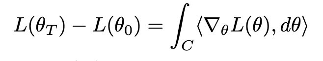
The change in loss from θ0 to θT may be calculated by integrating the dot product of the loss gradient and parameter motion along a path from θ0 to θT.
This then allows us to approximate the path integral using a series of first-order Taylor approximations-
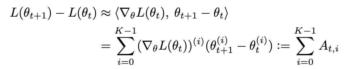
∇θL(θt) represents the gradient of the loss of the whole training set w.r.t. θ evaluated at θt, v(i)represents the i-th element of a vector v, and the parameter vector θ contains K elements.
This series is what defines LCA, since it allows us to index training steps and attribute changes in loss to each parameter.
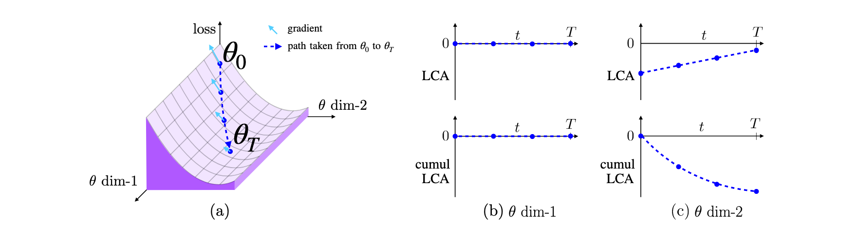
In this figure, the researchers showcase an example on a 2D loss surface (a). One parameter (θ dim-1) moves but does not affect the loss (b), while the other parameter (θ dim-2) moves in the negative gradient direction. By multiplying the parameter by its individual gradient movement, LCA can then be calculated.
As shown by this figure, a parameter that has a nonzero gradient and moves in the negative gradient direction has negative LCA, which indicates that it is helping **(since it is causing loss to decrease). Conversely, a parameter that has a nonzero gradient and moves in the positive gradient direction is **hurting (since it is causing loss to increase).
The researchers then tested their LCA methodology on two different tasks: a 3 layer FC network and LeNet model on the MNIST digits dataset, and a ResNet model on the Cifar-10 dataset. From their tests, they found three main insights:
-
Training is noisy: Some parameters help, some parameters hurt
-
Some layers go backwards: Even if the model is learning, some layers have positive cumulative LCA, indicating that they are going backwards.
-
Layers are synchronized: LCA trends seem to be in sync across layers in a model.
With these insights in mind, we decided to adapt the LCA code and see if we could replicate their results. Additionally, we wanted to build a simple workflow that would allow researchers to easily calculate LCA for their custom models.
We created our workflow based on a simple FC 3 layer network trained on MNIST. After looking at the Uber Research code, we realized that their workflow involved intermediate steps (training the model and downloading the weights, using the downloaded weights and calculating the gradients, using the calculated gradients and weights to calculate LCA), but this seemed cumbersome since it involved multiple programs and file downloads. We created our workflow to calculate LCA during model training and save to lists in-memory, allowing for immediate visualization. This is our code for calculating LCA and integrating it into our MNIST model:
Note that this is in Tensorflow 1.x; one of our to-do’s is to port this over to TensorFlow 2, as I’ll mention at the end of the post. But with this workflow, we are able to calculate LCA easily during model training, saving the LCA as a list for each layer.
Uber Research also provides plotting functions to visualize LCA, but we had to modify these a bit since we are calculating/storing LCA a little differently. Overall, these changes were minor; just changing the way that the underlying data was accessed. Here are some of the visualizations from our MNIST model:
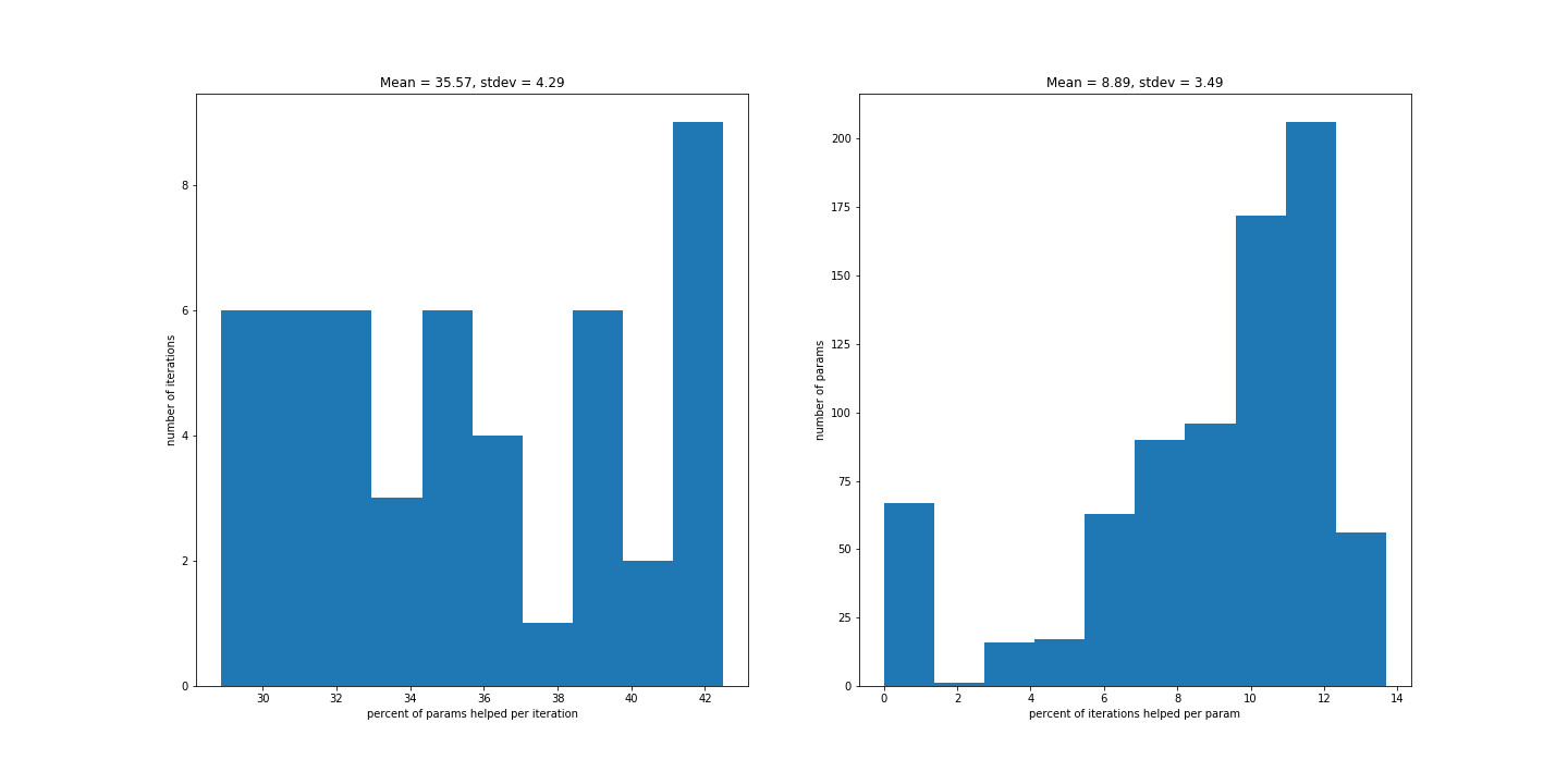 (Left) Percent of parameters that helped in each iteration. (Right) Percent of iterations that were helped by X number of parameters.
This visualization shows the variance in how parameters perform in our model, focused on the first layer. From the graph on the left, you can see that about 42% of parameters helped in most iterations, but this percentage ranged from 25–45%. The graph on the right tells a similar story; the number of parameters that helped in each iteration varied. This lines up with what was found by Uber Research (training is noisy).
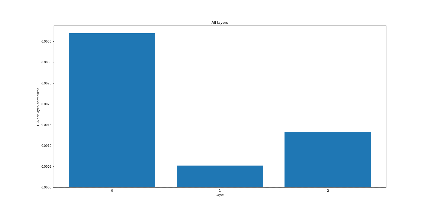 Cumulative LCA by layer
Interestingly, our model overall performs well after 50 iterations (~90% accuracy), but the net LCA for each layer was still slightly positive. Since our model learned overall, we would expect to see net negative LCA for our layers, since that would indicate that parameters overall helped more than they hurt. We have to look into this more, but the fact that these layers go backwards also lines up with the findings from the paper.
We also decided to test our LCA methodology on the APTOS 2019 Blindness Detection Dataset from Kaggle, which provides diabetic retinopathy images with labels. We didn’t change the structure of our model, but we wanted to explore LCA in a different task.
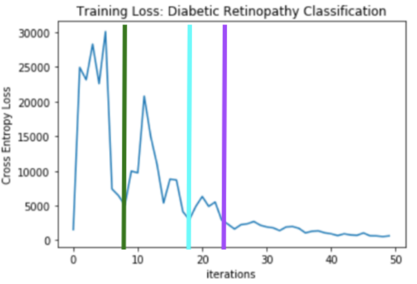
The graph above shows our training loss for the classification task, while the graph below shows the per-neuron cumulative LCA at each iteration, where red indicates negative LCA and green indicates positive LCA. The green, cyan, and magenta bars highlight three different moments in model training.
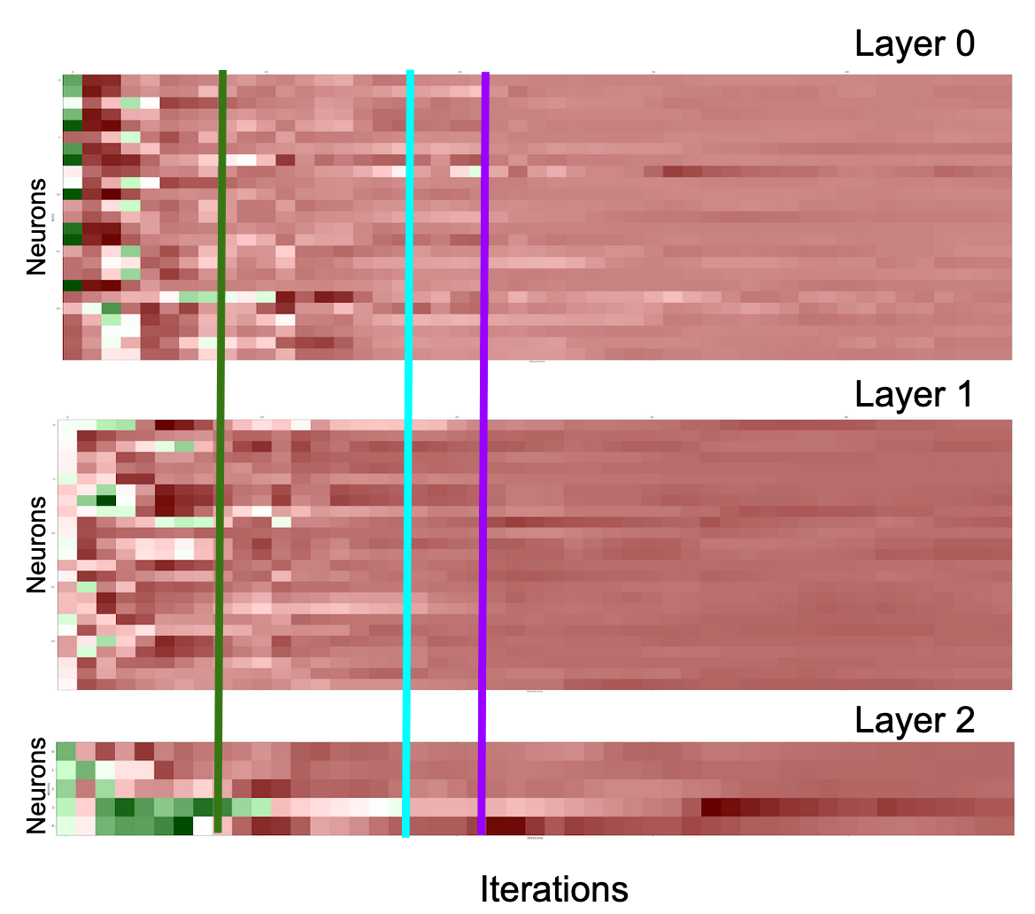
We can see that in the beginning, LCA is varied across the layers. But as the model learns, the neuronal LCA decreases in accordance with the loss. Layer 0 and 1 seem to be synchronized in their learning, while Layer 2 took a bit longer to stabilize. Overall, this method shows potential for understanding learning at a neuronal level, which can also inform model pruning and tuning.
Finally, since our ultimate goal was to adapt LCA for easy use in model training, we decided to integrate it with TensorBoard functionality, allowing someone to create these visualizations automatically while training their model. Currently, this was accomplished by calling the plotting functions during model training and saving the plot images to the buffer, where they can be accessed by TensorBoard.
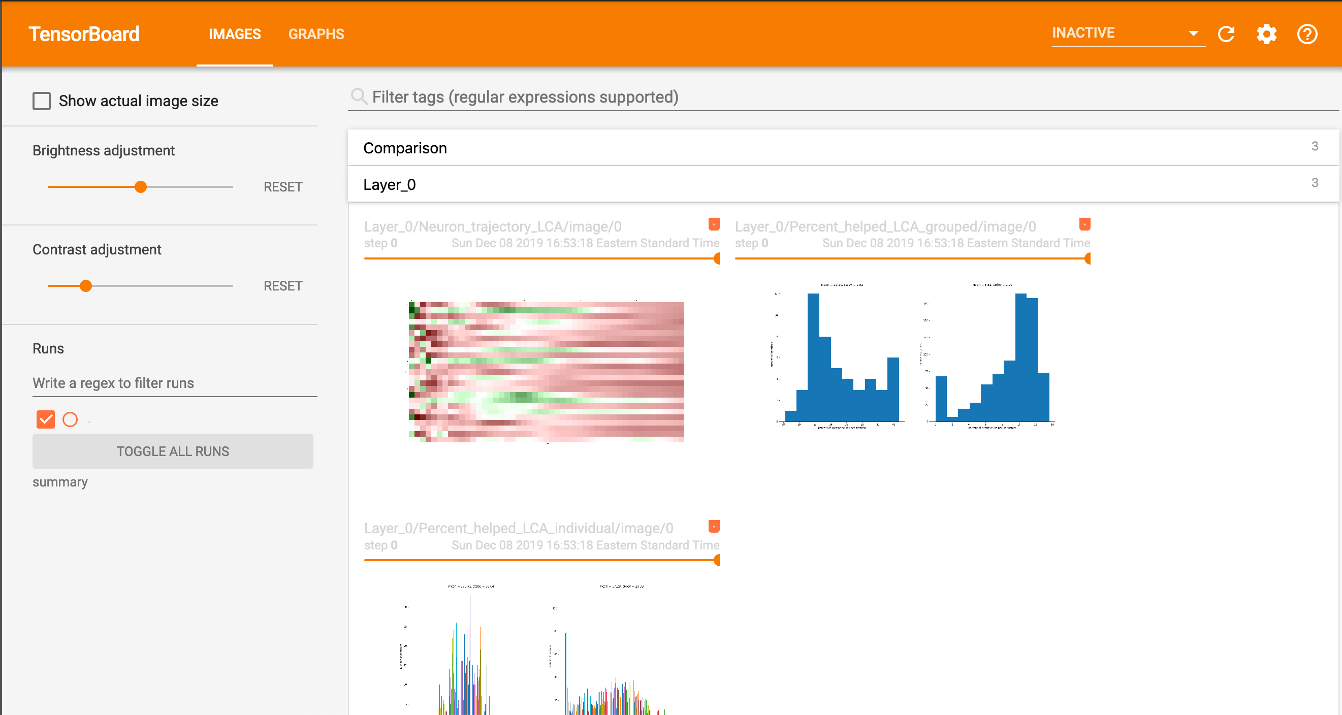
Ideally, we would like these images to be viewed dynamically by iteration, as opposed to their current static form. This is something that we’ll be working on next semester, now that we have the foundation built in.
Ultimately, this was a really interesting and rewarding project to build. Understanding how neural networks work behind-the-scenes continues to be an active area of research, and will only grow in importance as time goes on. The LCA approach is a great start in the right direction, and we hope that our simplified workflow can make it easier for researchers to tune and adjust their models based on this additional information. In the future, we hope to port over this workflow to Tensorflow 2.0, as well as potentially create a TensorBoard plug-in so that developers can easily visualize LCA in a callback.
Thanks to Uber Research for this awesome paper, and thank you for reading!
All code and slides are available on my Github repository.